Regularization: Bayesian’s Perspective

Introduction

Regularization is a fundamental concept in machine learning that helps prevent overfitting by adding a penalty term to the loss function. The most common types of regularization are Lasso (L1), Ridge (L2), and Elastic Net (a combination of L1 and L2).

Suppose we have a linear regression model:

$y_i = X_i^T\beta + \epsilon_i$ where $\epsilon_i \sim \mathcal{N}(0, \sigma^2)$.

Lasso (L1) Regularization is formulated as:

$\min_{\mathbf{\beta}} \frac{1}{n} \sum_{i=1}^{n} (\mathbf{\beta}^\intercal x_i - y_i)^2 + \lambda \|\mathbf{\beta}\|_1$

where $\|\mathbf{\beta}\|_1 = \sum_{j=1}^{p} |\beta_j|$ is the L1 norm of the weight vector; $\lambda$ is the regularization parameter that controls the strength of the penalty.

Ridge (L2) Regularization:

$\min_{\mathbf{\beta}} \frac{1}{n} \sum_{i=1}^{n} (\mathbf{\beta}^\intercal x_i - y_i)^2 + \lambda \|\mathbf{\beta}\|_2^2$

where $\|\mathbf{\beta}\|_2^2 = \sum_{j=1}^{p} \beta_j^2$ is the L2 norm of the weight vector; $\lambda$ is the regularization parameter that controls the strength of the penalty.

Elastic Net:

$\min_{\mathbf{\beta}} \frac{1}{n} \sum_{i=1}^{n} (\mathbf{\beta}^\intercal x_i - y_i)^2 + \lambda_1 \|\mathbf{\beta}\|_1 + \lambda_2 \|\mathbf{\beta}\|_2^2$

where the penalty terms are a combination of L1 and L2 norms, with $\lambda_1$ and $\lambda_2$ controlling the strength of each penalty.

When I first learned the concept and saw the formulations, the word ‘penalty’ made conceptual sense but little mathematical sense. I understand the intent to ‘penalize’ the model to help prevent overfitting. But why is it done by adding a penalty term consisting of the norm of the coefficients? How does it work mathematically?

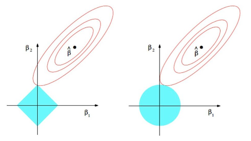
When searching for L1 and L2 regularization, one usually comes aross the following graph that shows the constraint regions for L1 and L2 regularization:

L1 and L2 regularization graphically represented. Source: Wikimedia Commons

The idea is the regularization term controls the values the coefficients can take. For L1 regularization, the constraint is a diamond-shaped region (the L1 norm), while for L2 regularization, the constraint is a circular region (the L2 norm). And because the L1 constraint has corners, it encourages sparsity in the coefficients, while the L2 constraint encourages small but non-zero coefficients.

Where do the constraint shapes come from? It turns out that according to optimization theory, the minimization problem with regularization terms can be reformulated as a constrained optimization problem. For example, the L1 regularization problem:

$\min_{\mathbf{\beta}} \frac{1}{n} \sum_{i=1}^{n} (\mathbf{\beta}^\intercal x_i - y_i)^2 + \lambda \|\mathbf{\beta}\|_1$

can be rewritten as:

${} {i=1}^{n} (^x_i - y_i)^2 $

subject to $\|\mathbf{\beta}\|_1 \leq B$

where $B$ is a constant that depends on $\lambda$. This means that the regularization term can be interpreted as a constraint on the coefficients, which leads to the specific shapes of the constraint regions.

The interpretation makes mathematical sense now. But the chain of thought - adding penalty terms -> reformulating as constrained optimization -> specific shapes of constraint regions - is long and not intuitive. For a long time, I try to remember the steps but still feel it’s a bit of a stretch. Until I came across the Bayesian interpretation of regularization.

Bayesian Rethinking

The idea of bayesian interpretation of regularization is simple: we are just telling the model, “Hey, let’s not get too excited about the data.”

The paradigm of Bayesian inference is about jointly considering the likelihood of the data and the prior beliefs of the coefficients, mathematically expressed as:

$P(\mathbf{\beta} | \mathbf{X}, \mathbf{y}) \propto P(\mathbf{y} | \mathbf{X}, \mathbf{\beta}) P(\mathbf{\beta})$

where $P(\mathbf{\beta} | \mathbf{X}, \mathbf{y})$ is the posterior distribution over the coefficients given the data, $P(\mathbf{y} | \mathbf{X}, \mathbf{\beta})$ is the likelihood of the data given the coefficients, $P(\mathbf{\beta})$ is the prior distribution over the coefficients.

Frequentists let the data speak for itself and find the best regression coefficients based on the likelihood function (a method called maximum likelihood estimation); whereas bayesians consider both the likelihood function and the prior distribution, saying, “Let’s not get too excited by the data, we put some boundaries on the coefficients based on our prior beliefs.” In fact, Frequentists’ approach is actually equivalent to using a uniform prior distribution in Bayesian’s framework, which means the coefficients are weighted equally and can take any value without any preference.

Why the ‘let the data speak for itself’ and ‘all coefficients are created equal’ approach is not ideal? Because the data can be noisy, and if we rely solely on the likelihood function, we might end up with coefficients that are too large or too small, or coefficientsthat only fit well with the dataset at hand but do not generalize well to new data. By incorporating a prior distribution that’s not uniform distribution, we have a leash to pull the coefficients back towards more reasonable values.

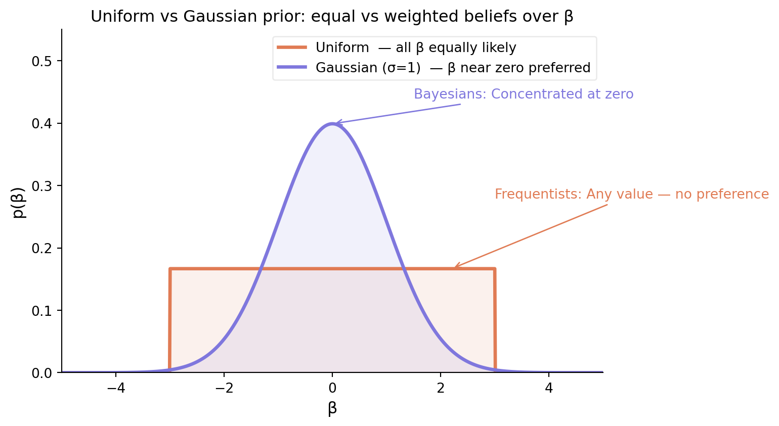
As shown on Figure.1, the uniform distribution, the probability of the coefficient being somewhere between -0.5 and 0.5 is the same as the probability of it being somewhere between 2 and 3. In contrast, the Gaussian distribution concentrates more probability mass around zero, which means we are saying, “We believe the coefficients should be near zero, but we are open to them being larger or smaller if the data strongly suggests it.”

Code

import numpy as np
import matplotlib.pyplot as plt
from scipy.stats import norm

x = np.linspace(-5, 5, 1000)

uniform = np.where((x >= -3) & (x <= 3), 1/6, 0)
gaussian = norm.pdf(x, scale=1.0)

fig, ax = plt.subplots(figsize=(8, 4.5))

ax.plot(x, uniform,  color="#E07B54", lw=2.5, label="Uniform  — all β equally likely")
ax.fill_between(x, uniform,  alpha=0.10, color="#E07B54")

ax.plot(x, gaussian, color="#7F77DD", lw=2.5, label="Gaussian (σ=1)  — β near zero preferred")
ax.fill_between(x, gaussian, alpha=0.10, color="#7F77DD")

ax.annotate(
    "Frequentists: Any value — no preference",
    xy=(2.2, 1/6), xytext=(3.0, 0.28),
    fontsize=10, color="#E07B54",
    arrowprops=dict(arrowstyle="->", color="#E07B54"),
)
ax.annotate(
    "Bayesians: Concentrated at zero",
    xy=(0, norm.pdf(0, scale=1.0)), xytext=(1.5, 0.44),
    fontsize=10, color="#7F77DD",
    arrowprops=dict(arrowstyle="->", color="#7F77DD"),
)

ax.set_xlabel("β", fontsize=12)
ax.set_ylabel("p(β)", fontsize=12)
ax.set_title("Uniform vs Gaussian prior: equal vs weighted beliefs over β", fontsize=12)
ax.legend(fontsize=10, framealpha=0.4)
ax.set_xlim(-5, 5)
ax.set_ylim(0, 0.55)
ax.spines[["top", "right"]].set_visible(False)

plt.tight_layout()
plt.show()

Uniform and Gaussian distributions on the same axes, showing how the Gaussian concentrates probability mass near zero while the uniform treats all values equally — Figure 1: Uniform vs Gaussian prior: equal vs weighted beliefs over β

The shape of the prior distribution corresponds to the type of regularization we are applying. For example, a Laplace prior leads to L1 regularization. On the other hand, a Gaussian prior leads to L2 regularization.

Posterior Formulation

The likelihood function for linear regression is given by:

$\mathcal{L}(Y|X, \beta) = \prod_{i=1}^{n} \frac{1}{\sqrt{2\pi}\sigma} \exp\left(-\frac{\epsilon_i^2}{2\sigma^2}\right) = \left(\frac{1}{\sqrt{2\pi}\sigma}\right)^n \exp\left(-\frac{1}{2\sigma^2}\sum_{i=1}^{n} \epsilon_i^2\right)$

The prior distribution over the coefficients $\beta$ can be defined as:

$P(\beta) = \prod_{j=1}^{p} P(\beta_j)$

where $P(\beta_j)$ is the prior distribution for each coefficient $\beta_j$.

The posterior distribution over the coefficients is then:

$P(\beta | X, Y) \propto \mathcal{L}(Y | X, \beta) P(\beta)$

$=\left(\frac{1}{\sqrt{2\pi}\sigma}\right)^n \exp\left(-\frac{1}{2\sigma^2}\sum_{i=1}^{n} \epsilon_i^2\right)*\prod_{j=1}^{p} P(\beta_j)$

Now we plug in the specific prior distributions for Lasso, Ridge, and Elastic Net to see how the posterior distribution leads to the regularization terms in the optimization problem.

Lasso

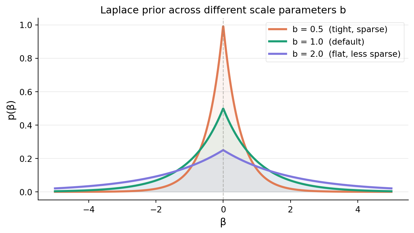
Lasso corresponds to a Laplace prior distribution:

$P(\beta) = \frac{1}{2b} \exp\left(-\frac{|\beta|}{b}\right)$

where $b$ is a scale parameter, $|\beta|$ is the absolute value of the coefficient.

Code

import numpy as np
import matplotlib.pyplot as plt

x = np.linspace(-5, 5, 1000)

params = [
    {"b": 0.5, "color": "#E07B54", "label": "b = 0.5  (tight, sparse)"},
    {"b": 1.0, "color": "#1D9E75", "label": "b = 1.0  (default)"},
    {"b": 2.0, "color": "#7F77DD", "label": "b = 2.0  (flat, less sparse)"},
]

fig, ax = plt.subplots(figsize=(7, 4))

for p in params:
    b = p["b"]
    density = (1 / (2 * b)) * np.exp(-np.abs(x) / b)
    ax.plot(x, density, color=p["color"], lw=2.5, label=p["label"])
    ax.fill_between(x, density, alpha=0.08, color=p["color"])

ax.axvline(0, color="#888780", lw=1, linestyle="--", alpha=0.5)

ax.set_xlabel("β", fontsize=12)
ax.set_ylabel("p(β)", fontsize=12)
ax.set_title("Laplace prior across different scale parameters b", fontsize=12)
ax.legend(fontsize=10, framealpha=0.4)
ax.spines[["top", "right"]].set_visible(False)
ax.grid(axis="y", alpha=0.25)

plt.tight_layout()
plt.show()

Three Laplace distributions with scale parameters b=0.5, b=1, and b=2, showing how larger b leads to a flatter, more spread out distribution while smaller b produces a sharper peak at zero — Figure 2: Laplace (double exponential) prior for b = 0.5, 1, 2

The joint prior distribution over all coefficients is:

$\prod_{j=1}^{p} P(\beta_j) = \prod_{j=1}^{p} \frac{1}{2b} \exp\left(-\frac{|\beta_j|}{b}\right)$

$= \left(\frac{1}{2b}\right)^p \exp\left(-\frac{1}{b}\sum_{j=1}^{p} |\beta_j|\right)$

Plugging this into the posterior distribution, we get:

$\mathcal{L}(Y | X, \beta) P(\beta) = \left(\frac{1}{\sqrt{2\pi}\sigma}\right)^n \exp\left(-\frac{1}{2\sigma^2}\sum_{i=1}^{n} \epsilon_i^2\right) * \left(\frac{1}{2b}\right)^p \exp\left(-\frac{1}{b}\sum_{j=1}^{p} |\beta_j|\right)$

= $\left(\frac{1}{\sqrt{2\pi}\sigma}\right)^n \left(\frac{1}{2b}\right)^p \exp\left(-\frac{1}{2\sigma^2}\sum_{i=1}^{n} \epsilon_i^2 - \frac{1}{b}\sum_{j=1}^{p} |\beta_j|\right)$

Now to find the maximum a posteriori (MAP) estimate of $\beta$, we take the log of the posterior distribution:

$\underbrace{\underbrace{nlog(\frac{1}{\sqrt{2\pi}\sigma}) + plog(\frac{1}{2b})}_{Constant} - \underbrace{(\frac{1}{2\sigma^2}\sum_{i=1}^{n} \epsilon_i^2 + \frac{1}{b}\sum_{j=1}^{p} |\beta_j|)}_{Minimize this}}_{In\ order\ to\ maximize\ this}$

Now the problem becomes:

$arg\min_{\beta} \left( \frac{1}{2\sigma^2}\sum_{i=1}^{n} \epsilon_i^2 + \frac{1}{b}\sum_{j=1}^{p} |\beta_j| \right)$

$=arg\min_{\beta} \frac{1}{2\sigma^2}\left( \sum_{i=1}^{n} \epsilon_i^2 + \frac{2\sigma^2}{b}\sum_{j=1}^{p} |\beta_j| \right)$

Since both $\sigma$ and $b$ are constants, we can ignore the $\frac{1}{2\sigma^2}$ term outside the brackets and use a new constant $\lambda$ to replace the term: $\lambda = \frac{2\sigma^2}{b}$.

Now we have:

$arg\min_{\beta} \left( \sum_{i=1}^{n} \epsilon_i^2 + \lambda\sum_{j=1}^{p} |\beta_j| \right)$

$=arg\min_{\beta} \left( RSS + \lambda\sum_{j=1}^{p} |\beta_j| \right)$

which is exactly the Lasso regularization formulation, with $\lambda = \frac{2\sigma^2}{b}$.

Therefore, the Lasso solutions are actually the maximum a posteriori (MAP) estimates of the coefficients under a Laplace prior distribution.

As we can see from Figure.2, the smaller $b$ gets, or equivamently, the larger $\lambda$ gets, the distribution gets a sharper peak at 0. In other words, the strongger the regularization parameter gets, the more the coefficients get pushed towards zero, encouraging sparsity in the coefficients.

Ridge

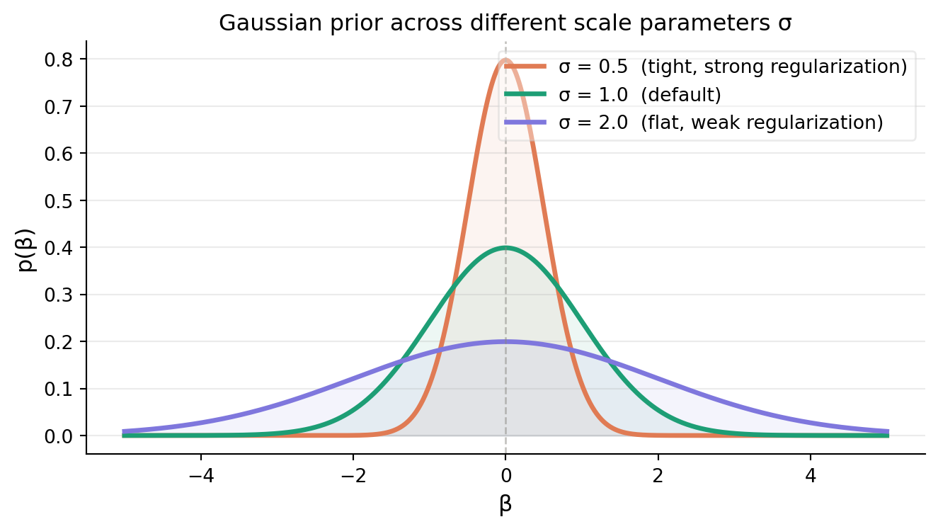
Ridge regularization corresponds to a Gaussian prior distribution for the coefficients:

\[ P(\beta) = \frac{1}{\sqrt{2\pi} \tau} \exp\left(-\frac{\beta^2}{2\tau^2}\right) \]

where $\tau^2$ is the variance parameter.

Code

import numpy as np
import matplotlib.pyplot as plt
from scipy.stats import norm

x = np.linspace(-5, 5, 1000)

params = [
    {"sigma": 0.5, "color": "#E07B54", "label": "σ = 0.5  (tight, strong regularization)"},
    {"sigma": 1.0, "color": "#1D9E75", "label": "σ = 1.0  (default)"},
    {"sigma": 2.0, "color": "#7F77DD", "label": "σ = 2.0  (flat, weak regularization)"},
]

fig, ax = plt.subplots(figsize=(7, 4))

for p in params:
    density = norm.pdf(x, scale=p["sigma"])
    ax.plot(x, density, color=p["color"], lw=2.5, label=p["label"])
    ax.fill_between(x, density, alpha=0.08, color=p["color"])

ax.axvline(0, color="#888780", lw=1, linestyle="--", alpha=0.5)

ax.set_xlabel("β", fontsize=12)
ax.set_ylabel("p(β)", fontsize=12)
ax.set_title("Gaussian prior across different scale parameters σ", fontsize=12)
ax.legend(fontsize=10, framealpha=0.4)
ax.spines[["top", "right"]].set_visible(False)
ax.grid(axis="y", alpha=0.25)

plt.tight_layout()
plt.show()

Three Gaussian distributions with scale parameters sigma=0.5, sigma=1, and sigma=2, showing how larger sigma leads to a flatter, more spread out distribution while smaller sigma produces a sharper peak at zero — Figure 3: Gaussian prior for σ = 0.5, 1, 2

With the same posterior formulation as in Lasso, we can plug in the Gaussian prior to get:

$\mathcal{L}(Y | X, \beta) P(\beta) = \left(\frac{1}{\sqrt{2\pi}\sigma}\right)^n \exp\left(-\frac{1}{2\sigma^2}\sum_{i=1}^{n} \epsilon_i^2\right) * \left(\frac{1}{\sqrt{2\pi} \tau}\right)^p \exp\left(-\frac{1}{2\tau^2}\sum_{j=1}^{p} \beta_j^2\right)$

To get the MAP estimate, we take the log of the posterior distribution:

$\underbrace{\underbrace{nlog(\frac{1}{\sqrt{2\pi}\sigma}) + plog(\frac{1}{\sqrt{2\pi} \tau})}_{Constant} - \underbrace{(\frac{1}{2\sigma^2}\sum_{i=1}^{n} \epsilon_i^2 + \frac{1}{2\tau^2}\sum_{j=1}^{p} \beta_j^2)}_{Minimize this}}_{In\ order\ to\ maximize\ this}$

Now the problem becomes:

$arg\min_{\beta} \left( \frac{1}{2\sigma^2}\sum_{i=1}^{n} \epsilon_i^2 + \frac{1}{2\tau^2}\sum_{j=1}^{p} \beta_j^2 \right)$

$=arg\min_{\beta} \frac{1}{2\sigma^2}\left( \sum_{i=1}^{n} \epsilon_i^2 + \frac{\sigma^2}{\tau^2}\sum_{j=1}^{p} \beta_j^2 \right)$

which is equivalent to:

$arg\min_{\beta} \left( RSS + \lambda\sum_{j=1}^{p} \beta_j^2 \right)$

where $\lambda = \frac{\sigma^2}{\tau^2}$.

Therefore, the Ridge solutions are the maximum a posteriori (MAP) estimates under a Gaussian prior.

From Figure.3, we can see that the smaller $\sigma$ gets, or equivalently, the larger $\lambda$ gets, the distribution gets more concentrated around zero.

Elastic Net

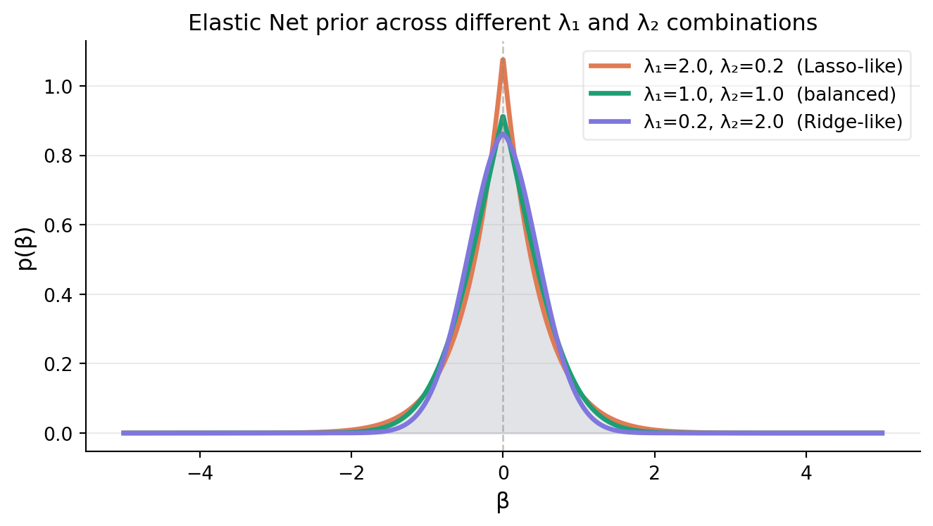
Elastic Net regularization, we use the product of Laplace and Gaussian prior distributions for the coefficients:

\[ P(\beta) = \frac{1}{2b} \exp\left(-\frac{|\beta|}{b}\right) * \frac{1}{\sqrt{2\pi} \tau} \exp\left(-\frac{\beta^2}{2\tau^2}\right) \]

$P(\beta) \propto \exp\left(-\frac{|\beta|}{b}-\frac{\beta^2}{2\tau^2}\right)$

Code

import numpy as np
import matplotlib.pyplot as plt

x = np.linspace(-5, 5, 1000)
dx = x[1] - x[0]

def elastic_net_prior(x, lambda1, lambda2):
    unnorm = np.exp(-lambda1 * np.abs(x) - lambda2 * x**2)
    return unnorm / (unnorm.sum() * dx)

params = [
    {"lambda1": 2.0, "lambda2": 0.2, "color": "#E07B54", "label": "λ₁=2.0, λ₂=0.2  (Lasso-like)"},
    {"lambda1": 1.0, "lambda2": 1.0, "color": "#1D9E75", "label": "λ₁=1.0, λ₂=1.0  (balanced)"},
    {"lambda1": 0.2, "lambda2": 2.0, "color": "#7F77DD", "label": "λ₁=0.2, λ₂=2.0  (Ridge-like)"},
]

fig, ax = plt.subplots(figsize=(7, 4))

for p in params:
    density = elastic_net_prior(x, p["lambda1"], p["lambda2"])
    ax.plot(x, density, color=p["color"], lw=2.5, label=p["label"])
    ax.fill_between(x, density, alpha=0.08, color=p["color"])

ax.axvline(0, color="#888780", lw=1, linestyle="--", alpha=0.5)

ax.set_xlabel("β", fontsize=12)
ax.set_ylabel("p(β)", fontsize=12)
ax.set_title("Elastic Net prior across different λ₁ and λ₂ combinations", fontsize=12)
ax.legend(fontsize=10, framealpha=0.4)
ax.spines[["top", "right"]].set_visible(False)
ax.grid(axis="y", alpha=0.25)

plt.tight_layout()
plt.show()

Four Elastic Net distributions showing how varying lambda1 and lambda2 shifts the prior between Laplace-like and Gaussian-like behaviour — Figure 4: Elastic Net prior for different λ₁ and λ₂ combinations

We proceed the same way as in Lasso and Ridge to get the MAP estimate of $\beta$ under the Elastic Net prior, which leads to the minimarzation problem:

$arg\min_{\beta} \frac{1}{2\sigma^2}\left(\sum_{i=1}^{n} \epsilon_i^2 + \frac{2\sigma^2}{b}\sum_{j=1}^{p} |\beta_j| + \frac{\sigma^2}{\tau^2}\sum_{j=1}^{p} \beta_j^2 \right)$

$=arg\min_{\beta}\left(RSS + \lambda_1\sum_{j=1}^{p} |\beta_j| + \lambda_2\sum_{j=1}^{p} \beta_j^2 \right)$

where $\lambda_1 = \frac{2\sigma^2}{b}$ and $\lambda_2 = \frac{\sigma^2}{\tau^2}$ are the regularization parameters for the L1 and L2 penalties, respectively.

Conclusion

We have shown how the regularization terms in Lasso, Ridge, and Elastic Net can be derived from a Bayesian perspective by considering different prior distributions over the coefficients. For me, the Bayesian perspective provides a more intuitive understanding of regularization: it allows us to make the model less sensitive to the data by pre-specifying a shape for the coefficient distributions.

References

E. Kamperi. Bayesian connection to Lasso and Ridge regression. 2020.
Q. Li and N. Lin. The Bayesian Elastic Net. Bayesian Analysis, 5(1), 151–170. 2010.
K. Weinberger. Empirical Risk Minimization. 2018.

Reuse

CC BY-SA 4.0

Citation

For attribution, please cite this work as:

Wang, Ray. 2026. “Regularization: Bayesian’s Perspective.” May 30. https://changruiraywang.com/blog/2026-05-30-bayesian-regularization/.