Learning about Gaussian Processes through the Lens of Regression and Stochastic Processes.
Author
Ray Wang
Published
June 14, 2026
Introduction
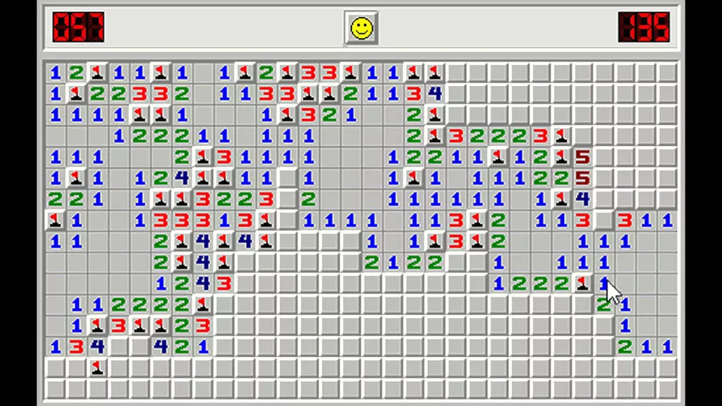
If you’re a millennial, chances are you played a Windows game called Minesweeper growing up. The premise is deceptively simple: a grid of covered squares hides a set number of mines, and your job is to uncover all the safe squares without triggering one. When you click a square, it either reveals a number — indicating how many of its neighboring squares contain mines — or ends the game in an explosion. Using those numbers, you reason about which adjacent squares are safe to click and which are likely deadly. The further you get, the more information you have, and the more confident your next move becomes. At its heart, Minesweeper is a game of inference under uncertainty. You build a mental model of where the mines are hiding, and you use it to decide where to step next.
A game of Minesweeper
Bayesian Optimization is the Minesweeper of Machine Learning (ML). A typical ML workflow involves defining an objective function — such as a loss function — and then solving for its minimum or maximum using numerical methods based on its derivatives. But there are cases where neither the objective function nor its derivatives are known. For such black-box functions, the only option is to draw samples in search of the optimal value. When samples are cheap to draw, a grid-search approach — systematically evaluating many combinations of input variables — works fine. But when samples are expensive, such as tuning the hyperparameters of a deep neural network or drilling for oil at candidate geographic coordinates, reaching the optimum with as few samples as possible becomes critical.
That is where Bayesian Optimization (BO) shines. BO consists of two components: a surrogate model — most commonly a Gaussian Process — and an acquisition function. The Gaussian Process is like the revealed squares on the Minesweeper grid, telling you what the landscape looks like around your observations. The acquisition function is your reasoning about where to click next. And the mines? They are the optimum values of your objective function.
Gaussian Processes (GP) through the Lens of Regression
There are many ways to introduce Gaussian Processes, of which the most intuitive to me is through the regression perspective.
Forget about Gaussian Processes for a minute. A typical regression workflow goes like this:
You use data to estimate regression parameters, then use the estimated parameters to make predictions. To estimate the regression parameters \(\mathbf{w}\), two paradigms are most common:
For inference tasks, the parameters are the most important since they embed the relationship between the predictors and the outcome. However, both methods lead to a single solution of \(\mathbf{w}\). In fact, there are many \(\mathbf{w}\) that may fit the data well and are worth considering. This argument is stronger for predictive tasks where the actual values of parameters \(\mathbf{w}\) are less of interest.
Bayesians say: let’s go directly from data to predictions, accounting for the variability of the parameters without having to estimate them:
This leads to the posterior predictive distribution:
\[P(y_i|x_i,D) = \int_w P(y_i|x_i,w,D)\,dw\]
The equation says: for a test point \(i\), we consider every possible value of the regression parameters and take a weighted average of their predicted values by integrating them out. The formula above can be further broken down into a product of the likelihood and posterior:
Here is where the magic happens. The likelihood \(P(y_i|x_i,w)\) is Gaussian. The posterior \(P(w \mid D) = \frac{P(D|w)P(w)}{z}\), if we assume a Gaussian prior \(P(w)\) (just like we do with Ridge regression), is also Gaussian. Two Gaussians multiplied together is still a Gaussian, so \(P(y|x,D)\) is also a Gaussian!
Now that is just one test case. We can extend the same idea to more than one test point:
Now the question becomes: how do we find \(\mu_{y_*|D}\) and \(\Sigma_{y_*|D}\)? The key assumption is that our training data and test data jointly follow a multivariate normal distribution (MVN):
\(K\) — an \(n \times n\) matrix of kernel evaluations between all pairs of training points, where entry \(K_{ij} = k(x_i, x_j)\). This is the covariance structure among the observed data.
\(K_*\) — an \(n \times 1\) vector of kernel evaluations between each training point and the test point \(x_*\), where entry \(K_{*i} = k(x_i, x_*)\). This is what links the training data to the test point.
\(K_*^T\) — the transpose of \(K_*\), a \(1 \times n\) vector. It appears in the lower left to keep the matrix symmetric, as a covariance matrix must be.
\(K_{**}\) — a scalar, the kernel evaluation of the test point with itself, \(k(x_*, x_*)\). This is the prior variance of the test point before seeing any data.
And what about Gaussian Processes? They are essentially MVN. The posterior predictive distribution can now be defined as follows (math derivation omitted):
In the example above, we treat the observed values \(y\) as the true values of the underlying function \(f\). However, in many applications this is not the case. The observed values are noisy, with an independent noise term layered on top:
\[\hat{Y}_i = f_i + \epsilon_i\]
In this case the covariance matrix becomes \(\hat{\Sigma} = \Sigma + \sigma^2\mathbf{I}\), and the Gaussian Process posterior distribution leads to:
To bring everything full circle: we bypass the estimation of regression parameters but are still able to make predictions. With some observed data, we can obtain a distribution for the values of the test data.
Yet the assumption and formulation can seem odd. Why combine training and test data? Why represent the covariance matrix with kernel functions? The core idea of GP is that data points close to each other should yield similar results. Under the GP framework, predictions are made by assuming all data come from the same generative model and examining how close the test data are to the training data via the kernel. It is analogous to estimating your house price based on the house prices in your neighborhood — without building a specific regression model with predictors like number of bedrooms or year built.
To think in MVN terms is a paradigm shift. In most regression settings, individual data points are assumed to have their own distributions. In Gaussian Processes, our data are counted only as a partial observation of one sample from an MVN. To facilitate understanding, we now visit the origin of Gaussian Processes in Stochastic Processes.
Gaussian Processes (GP) through the Lens of Stochastic Processes
By Wikipedia, a Gaussian Process is a time continuous stochastic process \(\{X_t; t \in T\}\) such that for every finite set of indices \(t_1, \ldots, t_k\) in the index set \(T\),
is a multivariate Gaussian random variable. Essentially, GP observations are never independent — although collected at different inputs, they are jointly Gaussian, correlated with each other through the kernel function. The data points collectively are one realization from the joint distribution:
The covariance structure encoded in \(K\) means that observing \(f(x_i)\) says something about \(f(x_j)\) for nearby \(x_j\). The most common choice for the covariance structure is the Radial Basis Function (RBF) kernel:
We have now discussed two views of Gaussian Processes. The Conditional View: after observing some points, the remaining points follow an updated Gaussian — the posterior predictive distribution from the regression perspective. And the Joint View: all observations together are one draw from a multivariate Gaussian, corresponding to the stochastic process perspective.
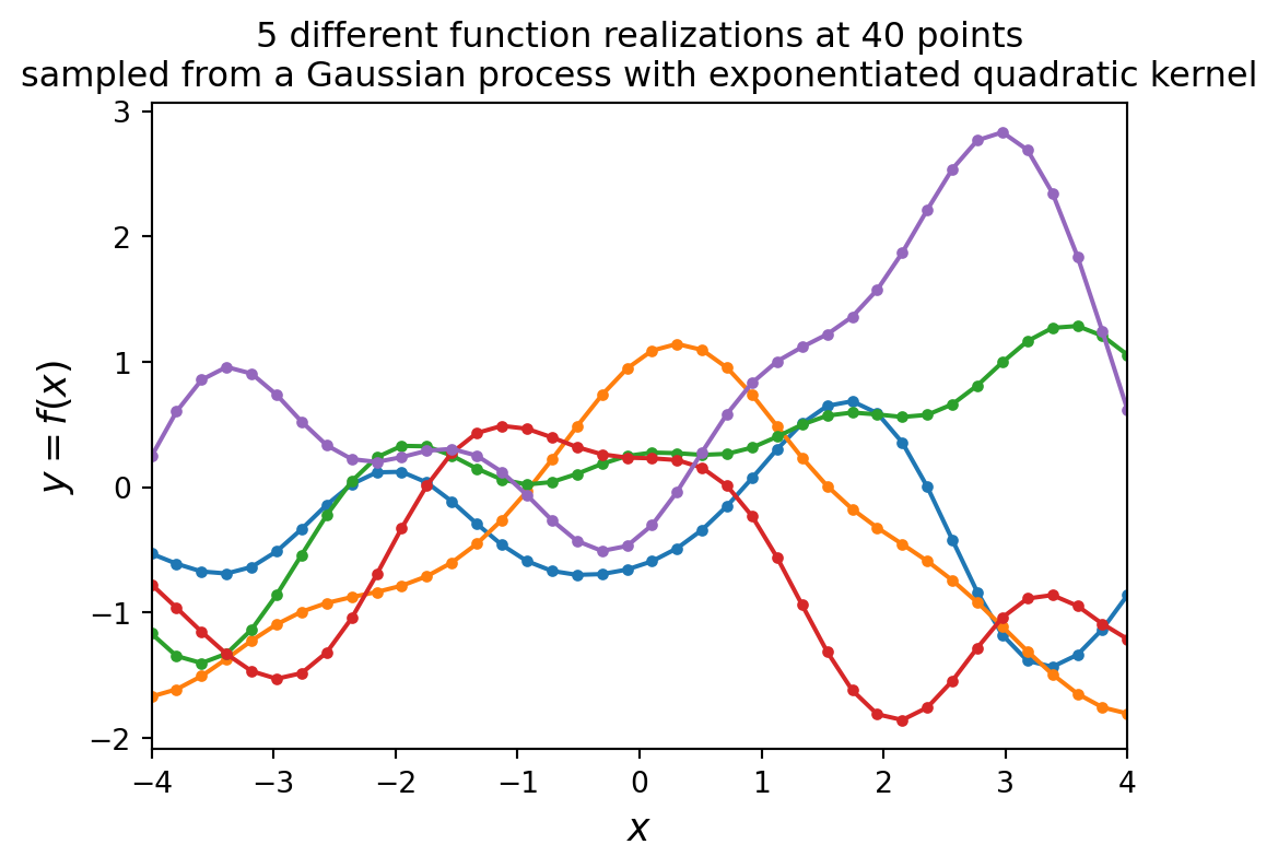
In this section, we code GPs in Python to generate plots of both views using the RBF kernel.
Code
import numpy as npimport scipyimport scipy.spatial.distanceimport itertoolsimport matplotlib.pyplot as pltimport matplotlib.gridspec as gridspecfrom matplotlib.figure import Figurefrom matplotlib.gridspec import SubplotSpecfrom mpl_toolkits.axes_grid1 import make_axes_locatablefrom numpy import ndarray as KernelMatrixfrom scipy.stats.qmc import LatinHypercube
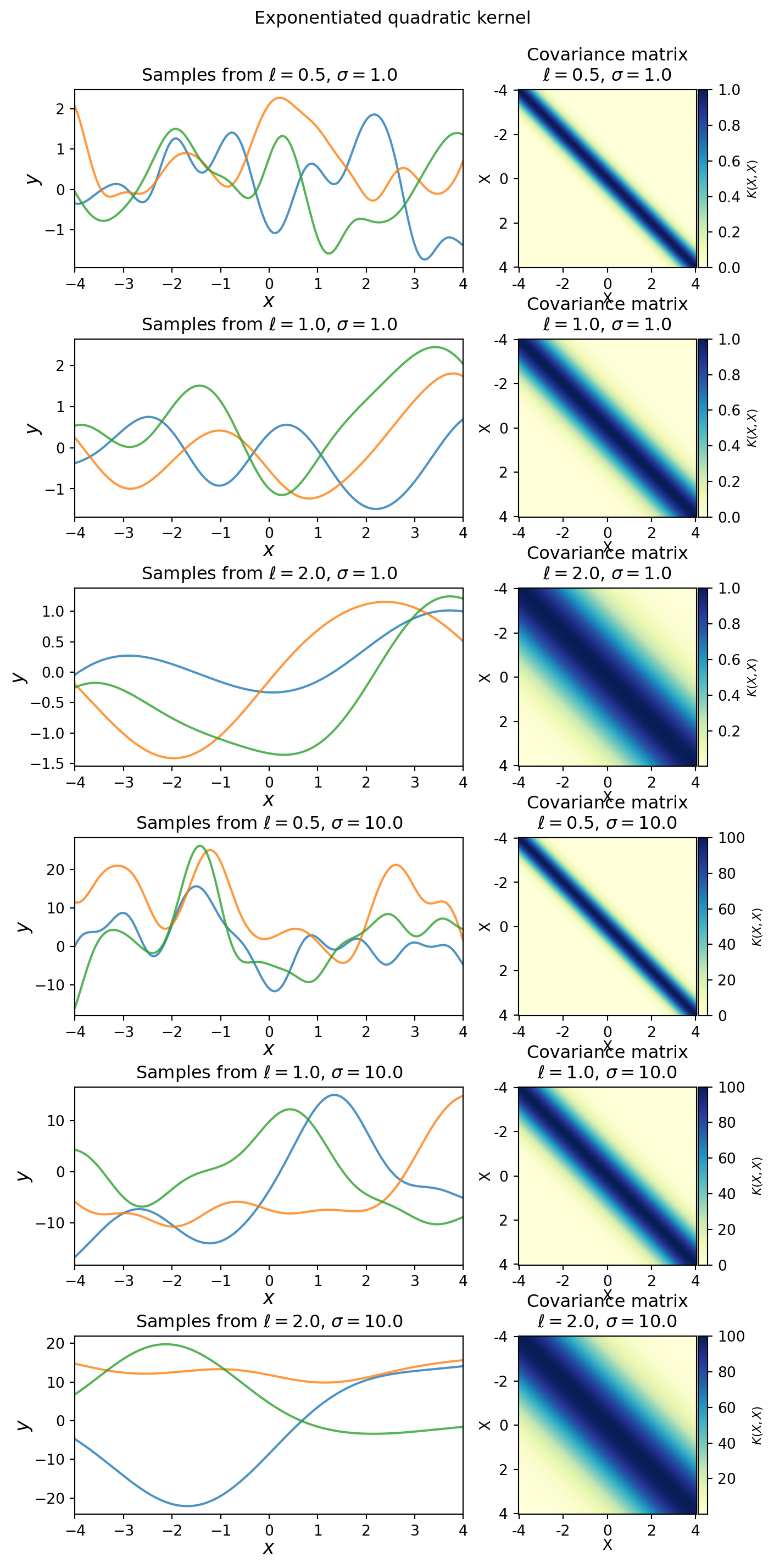
Each curve below represents one GP sample, with 40 observed points shown and infinitely many unobserved points implied. One collection of 40 data points is only a partial observation of one realized function.
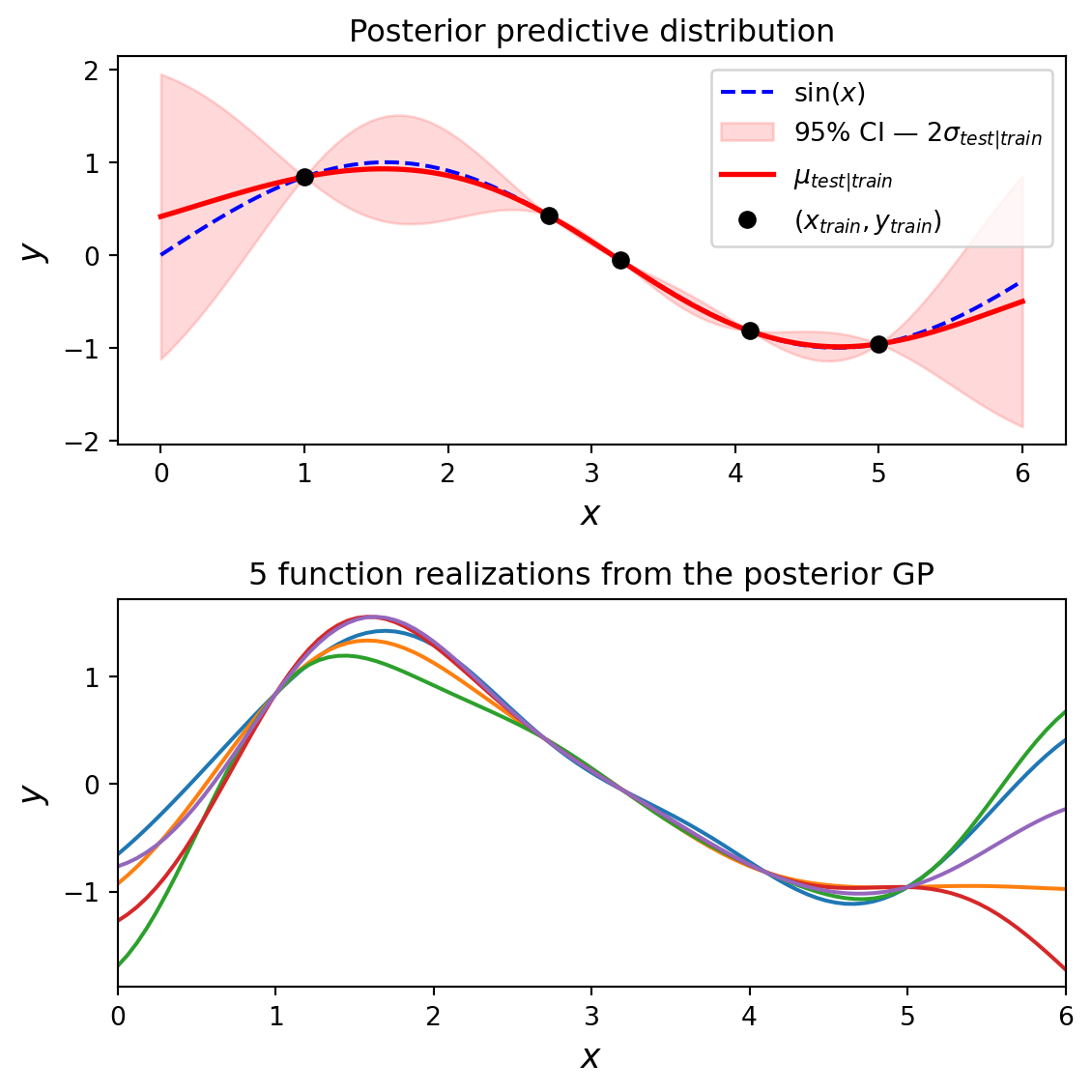
Conditional View — Posterior Predictive Distribution
Suppose we have a function \(f(x) = \sin(x)\) for which we have observed the values at several data points, and we hope to build a posterior predictive distribution over the entire space. Plugging the observed values into the posterior predictive formula:
The characteristic football/sausage shape reflects low variance around observed values and high variance for points far from the training data. Statistically, 95% of samples drawn from the posterior should fall within the shaded 95% confidence interval.
Why Conditioning Reduces Variance
With a GP, the closer \(x_*\) is to the training points, the more confident the model becomes, and thus the more variance gets reduced. But why? What role does the kernel play? Let’s unpack the math behind the posterior covariance.
The posterior covariance of a test point \(x_*\) given training data is:
\[\Sigma_{y_*|D} = K_{**} - K_*^T K^{-1} K_*\]
where \(K_{**}\) is the prior variance of \(x_*\) — the uncertainty before seeing any data — and \(K_*^T K^{-1} K_*\) is the variance removed by the training points. Assume \(n\) training points and a single test point \(x_*\), with \(K\) as \(n \times n\), \(K_*\) as \(n \times 1\), and \(K_*^T\) as \(1 \times n\). The full product is a scalar:
Given the positive definite nature of kernels, this quantity is always positive — it can be thought of as the total amount of variance removed from the test data.
To see how much variance is removed, let’s examine the quantity with three training points \((x_1, x_2, x_3)\) and one test point \(x_*\). Set \(a = k(x_*, x_1)\), \(b = k(x_*, x_2)\), \(c = k(x_*, x_3)\), with \(m_{ij}\) denoting entries of \(K^{-1}\):
\[K_*^T K^{-1} K_* = \begin{bmatrix} a & b & c \end{bmatrix}
\begin{bmatrix} m_{11} & m_{12} & m_{13} \\ m_{21} & m_{22} & m_{23} \\
m_{31} & m_{32} & m_{33} \end{bmatrix}
\begin{bmatrix} a \\ b \\ c \end{bmatrix}
= m_{11}a^2 + m_{22}b^2 + m_{33}c^2 + 2m_{12}ab + 2m_{13}ac + 2m_{23}bc\]
The squared terms\(a^2, b^2, c^2\) capture how similar \(x_*\) is to each individual training point. The cross terms\(ab, ac, bc\) capture interactions between \(x_*\)’s relationships to different training points and are treated as constants driven by the training data structure.
With the RBF kernel, each similarity score \(k(x_*, x_i)\) approaches 1 when \(x_*\) is close to \(x_i\) and 0 when far away. This means one nearby training point gives moderate variance reduction; two nearby training points give larger reduction; and no nearby training points means the GP falls back to its prior. The variance reduction is therefore a vote from each training point, weighted by proximity to \(x_*\). GP uncertainty is locally determined — confidence builds up around observed points and fades in unexplored regions. As we will see in the second blog of the series, this is exactly the signal the acquisition function uses to decide where to sample next.
Higher Dimension GP
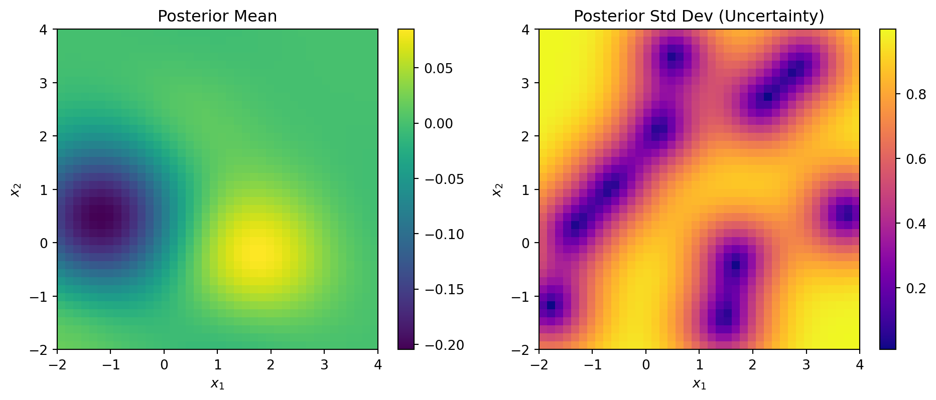
So far we have focused on simple 1D examples. In the real world, data points come in much higher dimensions. The distance calculation remains the same: for each pair of data points, we take the distances across each feature and compute the norm of the difference vector. The example below extends the GP to a 2D input space, modeling the underlying function \(f(x_1, x_2) = x_1 \exp(-x_1^2 - x_2^2)\).
The posterior mean (left) shows the GP’s best estimate of the underlying function across the 2D input space. The color intensity represents the predicted function value — warmer colors indicate higher values, cooler colors indicate lower values. The surface is smooth, as expected from the RBF kernel.
The posterior uncertainty (right) shows the posterior standard deviation \(\sigma_{test|train}\) at each test point — the square root of the diagonal of \(\Sigma_{y_*|D}\). Dark regions indicate low uncertainty near the 10 Latin Hypercube training points, where variance reduction is large. Bright regions indicate high uncertainty far from all training points, where the posterior falls back toward the prior. With only 10 training points over a 2D space, large portions of the input space remain uncertain — illustrating precisely why efficient sampling strategies like BO matter when evaluations are expensive.
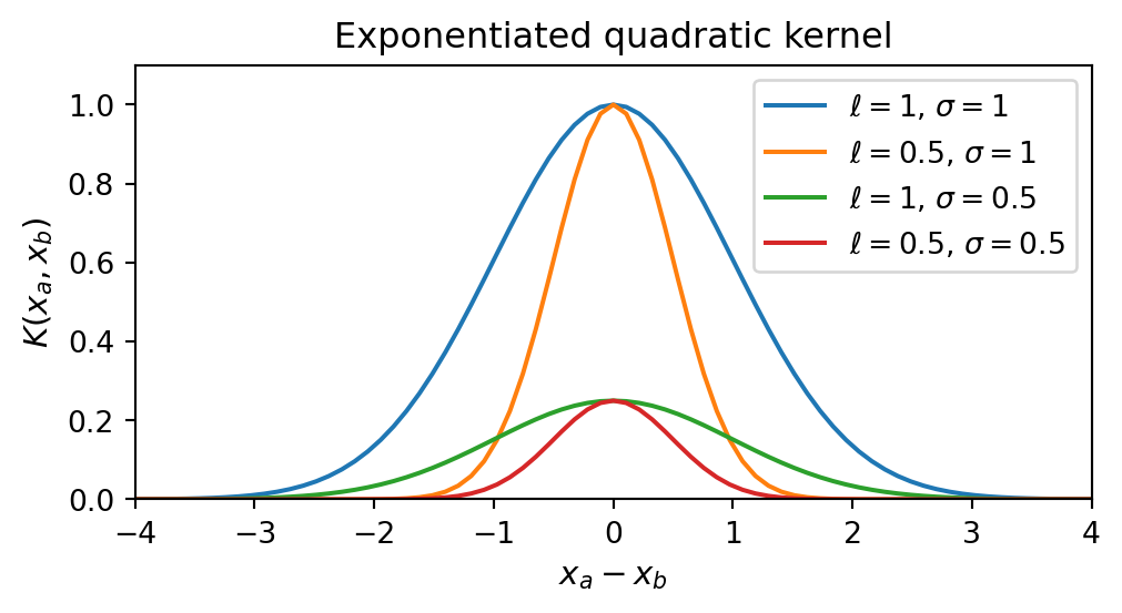
where two hyperparameters are required: \(\sigma\) (amplitude) and \(\ell\) (lengthscale). In practice, these parameters are unknown and usually estimated via Maximum Likelihood Estimation. A great reference is Gaussian processes (2/3) — Fitting a Gaussian process kernel.
Each parameter affects the shape of the kernel function and the resulting GP. Let’s first look at how the parameters affect the kernel function itself:
The RBF kernel has two hyperparameters: the length scale \(\ell\) and the amplitude \(\sigma\). The six plots above correspond to all combinations of \(\sigma \in \{1, 10\}\) and \(\ell \in \{0.5, 1, 2\}\), generated by itertools.product in this order:
Plot
\(\sigma\)
\(\ell\)
1
1.0
0.5
2
1.0
1.0
3
1.0
2.0
4
10.0
0.5
5
10.0
1.0
6
10.0
2.0
Length scale \(\ell\) controls the smoothness of the function. At \(\ell = 0.5\) (plots 1, 4), the sampled functions are highly wiggly — only points within 0.5 units of each other are considered similar, so the function changes direction rapidly. At \(\ell = 1\) (plots 2, 5), functions are smooth at a moderate pace. At \(\ell = 2\) (plots 3, 6), the functions are very slow-moving — points up to 2 units apart remain highly correlated, producing long sweeping curves. In the covariance matrix, a larger \(\ell\) spreads correlations further from the diagonal, making the matrix appear more uniformly bright. A smaller \(\ell\) concentrates correlation near the diagonal.
Amplitude \(\sigma\) controls the vertical scale of the function. At \(\sigma = 1\) (plots 1–3), function values stay roughly within \([-1, 1]\). At \(\sigma = 10\) (plots 4–6), they can swing as wide as \([-10, 10]\), while the smoothness pattern mirrors plots 1–3 exactly since \(\ell\) is unchanged. Comparing plot 1 (\(\ell=0.5\), \(\sigma=1\)) to plot 4 (\(\ell=0.5\), \(\sigma=10\)): identical wiggliness, but the vertical range is inflated by a factor of 10. \(\sigma\) scales the entire kernel matrix by \(\sigma^2\), inflating variance at every point without touching the correlation structure. Think of \(\ell\) as controlling the shape of the functions and \(\sigma\) as controlling their range.
Conclusion
Gaussian Processes are a powerful and elegant tool for modeling uncertainty. Starting from the regression perspective, we saw how integrating out the parameters leads naturally to the posterior predictive distribution — a Gaussian whose mean and covariance are fully defined by the kernel function. From the stochastic processes perspective, we saw that a GP treats the entire function as a single draw from a multivariate Gaussian, where observations are jointly correlated rather than independent.
The kernel function is the engine of the GP. It encodes how information propagates from observed points to unobserved ones. The closer a test point is to the training points, the more confident the model becomes, and the more variance gets reduced. This variance reduction is not magic — it is a weighted sum of similarities, driven entirely by how close a test point is to the training data.
Back to the Minesweeper analogy: the GP is your mental model of the board. Each observation updates your belief about the surrounding landscape, narrowing uncertainty near revealed squares and leaving it wide open in unexplored corners. In the next blog of the series, we will see how the acquisition function uses that uncertainty map to decide where to click next — and how the full Bayesian Optimization loop comes together.