Introduction
Just like backpropagation is the primitive mathematical engine of AI, kernels are the underlying mechanism of many powerful machine learning algorithms. In fact, the concept of kernels is so fundamental that it can still be found in today’s AI applications, although in a more implicit way.
Despite its importance, the concept of kernels is probably one of the most confusing and thus most underappreciated topics in machine learning. Most data practitioners, like myself, first learned of kernels in the context of Support Vector Machines (SVM), which itself is another hard topic. On the other hand, if you try to learn kernel from its mathematical definition which involves Hilbert spaces, you will easily get lost.
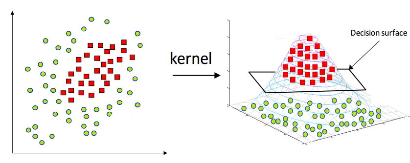
One of the most common interpretation one can find online is that kernels are a way to implicitly map data into a high-dimensional feature space, which allows us to capture complex relationships in the data (shown as Figure.1). While this interpretation is intuitive, it only explains the necessity to go to high-dimension, but does not explain what role kernels have to play in the process.
In this blog, I try to retell the story of kernels based on my learning notes of many amazing resources, explaining what they are, why they are important, and how they work in the context of machine learning algorithms.
What are Kernels?
Intuitively speaking, a kernel function \(K(x,y)\) is a similarity function. It takes two data points as input and returns a number that measures the similarity between the two data points. The similarity measure is calculated based on the inner product of the features of the two data points. The more similar the two data points are, the higher the kernel value. Moreover, which is more important, the similarity is achieved very cost-effectively.
So kernels do only one thing, and they do it extremely well: measuring similarities between two data points with minimal computational overhead.
As a toy example, consider a person’s height and weight as a two-dimension feature vector:
\(\mathbf{x}=(x_1,\ x_2)\)
where \(x_1\) is height and \(x_2\) is weight.
Suppose we have two people \(\mathbf{x}\) and \(\mathbf{z}\) with feature vectors \((180, 70)\) and \((160, 50)\), and we want to calculate their similarity:
\(\langle \mathbf{x},\mathbf{z} \rangle= x_1*z_1+x_2*z_2 = 180 \times 160 + 70 \times 50\)
Now suppose there is a non-linear, high-dimension feature vector transformed from the original feature vector, that measures the similarity in a more complex way by including the square and interaction terms:
\[\phi(\mathbf{x}) = (x_1^2,\ x_2^2,\ \sqrt{2}\,x_1 x_2)\]
where \(\phi(\mathbf{x})\) is the transformed feature vector.
The inner product of two feature vectors becomes:
\[\langle \mathbf{x}, \mathbf{z} \rangle = 180^2 \cdot 160^2 + 70^2 \cdot 50^2 + \sqrt{2} \cdot 180 \cdot 70 \cdot \sqrt{2} \cdot 160 \cdot 50 = 1{,}043{,}290{,}000\]
Notice that this computation calculates the transformed non-linear terms first, then add them up, which is 11 multiplications and 2 summations in total.
However, there actually exists a function that does not require the actual calculation of the transformed high-dimension features and thus makes the computation easier:
\[K(\mathbf{x}, \mathbf{z}) = (\langle \mathbf{x}, \mathbf{z} \rangle)^2 = (x_1 z_1 + x_2 z_2)^2 = (180 \times 160 + 70 \times 50)^2 = 1{,}043{,}290{,}000\]
The function takes the inner product of the original feature vector and returns the same value. It only takes 3 multiplications and 1 summation — same result, far less computation.
To recap, with the first approach, we have to square and multiply the high-dimension terms: \(x_1^2,x_2^2,z_1^2,z_2^2,x_1 x_2 z_1 z_2\). However, with the second approach, we don’t need such high-dimension terms. We only need the low-dimension terms: \(x_1x_2,z_1z_2\). The two approaches give the same result, but the second approach is much more computationally efficient.
In math’s language, the function \(K\) is called a kernel function. It takes low-dimension features as input and returns the inner product of high-dimension features, skipping the step of calculating high-dimension features and their inner product. As an illustration, the kernel approach vs the non-kernel approach can be visualized as:
Low-dimension feature → kernel function with low-dimension features → high-dimension inner product
Low-dimension feature → high-dimension features → high-dimension inner product
The fact that the kernel function allows us to access high-dimension inner product using only low-dimension features is called the ‘Kernel Trick’.
Why Kernels?
The idea of efficient computation of inner products in high-dimension feature spaces is not just a mathematical curiosity. It has profound implications for machine learning algorithms.
In Machine Learning, it is a common feature engineering practice to create more features from existing features. Think of all the non-linear interaction terms: two-way interactions, three-way interactions, and even higher way interactions. To take it to the extreme, one could add as many non-linear terms as possible, with the hope that the practice reveals hidden relationships among the data. That is where Kernels come into play.
Two facts make kernels extremely powerful in machine learning:
(1). Computational Convenience - The transformation of data from low dimension to high dimension in the form of inner products of data points.
(2). Kernelized Algorithms - Some machine learning algorithms can actually take inner products of data points as input, making it possible to benefit from the computational effectiveness offered by kernels.
We go through the example of linear regression to illustrate both points.
Kernelized Linear Regression
It turns out that the conventional linear regression model can be re-expressed as a linear combination of inner products of input feature vectors.
Imagine a linear regression model with p features. Denote the regression parameter vector as \(\mathbf{w}\). The loss function is:
\[\ell(\mathbf{w}) = \sum_{i=1}^{n} (\mathbf{w}^T x_i - y_i)^2\]
where \(x_i\) is the feature vector of the ith observation, e.g. \[\begin{pmatrix} x_{i1} \\ x_{i2} \\ \vdots \\ x_{ip} \end{pmatrix}\].
Gradient descent updates \(\mathbf{w}\) as:
\[w_{t+1} = w_t - s \left(\frac{\partial \ell}{\partial \mathbf{w}}\right)\]
where \(s\) is the learning rate.
Here, \(\frac{\partial \ell}{\partial \mathbf{w}} = 2\sum_{i=1}^{n}(\mathbf{w}^T \mathbf{x}_i - y_i)\)
Therefore, the gradient can be expressed as a linear combination of input feature vectors:
\[\frac{\partial \ell}{\partial \mathbf{w}} = \sum_{i=1}^{n} \underbrace{2(\mathbf{w}^T \mathbf{x}_i - y_i)}_{\gamma_i} \mathbf{x}_i = \sum_{i=1}^{n} \gamma_i \mathbf{x}_i\]
Now that’s one tiny step along the gradient descent process. Since the parameters \(\mathbf{w}\) are essentially many of those tiny steps added together, it’s intuitive to think of the parameters \(\mathbf{w}\) as a linear combination of input feature vectors:
\[\mathbf{w} = \sum^{J}_j\sum_{i=1}^{n} \gamma_i \mathbf{x}_i = \sum_{i=1}^{n} \alpha_i \mathbf{x}_i\]
where \(J\) is the total steps of gradient descent; \(\alpha_i\) is the new weights of the ith feature vector \(x_i\) after combining J rounds of \(\gamma_i\).
The equation above is a very important representation of the linear regression model. It shows that the regression parameters \(\mathbf{w}\) can be expressed as a linear combination of the input feature vectors:
$$ _{i=1}^{n} _i _i=
1 {1st observation} + 2 {2nd observation} + + n {nth observation} = \[\begin{pmatrix} \hat{w}_1 \\ \hat{w}_2 \\ \vdots \\ \hat{w}_p \end{pmatrix}\]$$
A huge benefit of the representation is that we can now just do the gradient descent in terms of \(\alpha\), which is of dimension \(n\times 1\):
\[ \mathbf{w}^1 = \sum_{i=1}^{n} \alpha_i^0 \mathbf{x}_i - s \sum_{i=1}^{n} \gamma_i^0 \mathbf{x}_i = \sum_{i=1}^{n} (\alpha_i^0 - s\gamma_i^0) \mathbf{x}_i = \sum_{i=1}^{n} \alpha_i^1 \mathbf{x}_i \]
If we do gradient descent on the parameters themselves, the dimension could be as high as \(2^d \times 1\).
Under the new representation, however, the regression model can be re-expressed as taking the inner product between data points as input:
\[y_j = w^Tx_j + b = \sum_{i=1}^n\alpha_i \underbrace{x_ix_j^T}_{K_{ij}}+b\]
where \({K_{ij}}\) is the kernel function between the ith and jth observation.
To recap, we’ve shown that the linear regression model can be rewritten as a function of inner products of pairs of observations.
Now if we want to make a prediction for an observation \(\mathbf{z}\), the prediction can be made via:
\[h(\mathbf{z}) = \mathbf{w}^T \mathbf{z} + b = \sum_{i=1}^{n} \alpha_i x_i^T \mathbf{z} + b\]
where \(x_i^T \mathbf{z}\) is the inner product between the ith observation’s feature vector \(x_i^T\) \((1 \times p)\) and the new observation’s feature vector \(\mathbf{z}\) \((p \times 1)\).
We are essentially taking the inner product between the new observation with each of the existing observations. And since \[\underbrace{\mathbf{x}_i^\top}_{\scriptsize(1 \times p)} \underbrace{\vphantom{\mathbf{x}_i^\top}\mathbf{z}}_{\scriptsize(p \times 1)}\] returns a number \(1 \times 1\), we add up the results according to their weights \(\alpha\).
Computational Convenience
Everything looks good so far. But why do we want to re-express the linear regression model as a function of inner products of pairs of observations?
Well, with the original linear regression model, if we want to include as many non-linear features as possible, the number of features will grow exponentially with the number of original features, making it computationally expensive.
Suppose we have a d-dimensional feature vector \(\mathbf{x}\) to start with:
\[\mathbf{x} = \begin{pmatrix} x_1 \\ \vdots \\ x_d \end{pmatrix}\]
where \(x_1\) through \(x_d\) represent the features of an observation. For example, if an observation represents a house, \(x_1\) could be area, \(x_2\) could be year built, \(x_3\) could be number of bedrooms, etc.
To capture non-linear relationships, we can then have a transformation \(\phi(x)\) such that:
\[\phi(x) = \begin{pmatrix} x_1 \\ \vdots \\ x_d \\ x_1x_2 \\ \vdots \\ x_{d-1}x_d \end{pmatrix}\]
With a feature vector of length \(d\), a transformation \(\phi(x)\) that contains all possible interaction terms is of length \(2^d\). There are two problems with this approach:
(1). The number of features grows exponentially with the number of original features, making it computationally expensive to calculate the regression parameters.
(2). The inner product of two transformed observations \(\phi(\mathbf{x})^\top \phi(\mathbf{z})\) is also computationally expensive to calculate, since the dimension of the transformed feature vector \(\phi(x)\) is \(2^d\).
The kernelized form of the linear regression model, however, allows us to bypass both problems.
First, with the kernelized form, the number of regression parameters is just \(n\), since each observation gets their own weight \(\alpha_i\).
Second, there is a kernel function that allows us to calculate the inner product of two transformed observations \(\phi(\mathbf{x})^\top \phi(\mathbf{z})\) without actually calculating the transformed features:
\[K(\mathbf{x}, \mathbf{z}) = \phi(\mathbf{x})^\top \phi(\mathbf{z}) = 1 \cdot 1 + x_1 z_1 + x_2 z_2 + \cdots + x_1 x_2 z_1 z_2 + \cdots + x_1 \cdots x_d z_1 \cdots z_d = \prod_{k=1}^{d} (1 + x_k z_k)\]
So instead of calculating the high-dimension features one by one, we can directly get the inner product of the high-dimension features by calculating the kernel function with the original low-dimension features.
Therefore, by re-expressing the linear regression model as a function of inner products of pairs of observations, we can not only estimate the parameters more efficiently but also capture complex non-linear relationships in the data.
Types of Kernels
There are many types of kernels, and the choice of which kernel to use depends on the specific problem and data at hand. The most commonly used kernels are Polynomial and Radial Basis Function (RBF) Kernel.
Polynomial Kernel
The kernel from the linear regression example is actually a type of Polynomial kernel:
\[\textbf{Polynomial:} \quad K(\mathbf{x}, \mathbf{z}) = (1 + \mathbf{x}^\top \mathbf{z})^d\]
Suppose observation \(x\) has two features \(x_1\) and \(x_2\):
\[x = \begin{pmatrix} x_1 \\ x_2 \end{pmatrix}\]
We want to add a bias term plus the square and interaction terms:
\[\phi(x) = \begin{pmatrix} 1 \\ x_1 \\ x_2 \\ x_1 x_2 \\ x_1^2 \\ x_2^2 \end{pmatrix}\]
The inner product of two transformed observations is:
\[\langle \phi(\mathbf{x}), \phi(\mathbf{z}) \rangle = 1 + x_1 z_1 + x_2 z_2 + x_1 x_2 z_1 z_2 + x_1^2 z_1^2 + x_2^2 z_2^2\]
This is equivalent to the 2nd degree polynomial kernel:
\[K_{\text{poly}(2)}(\mathbf{x}, \mathbf{z}) = (1 + \mathbf{x}^T \mathbf{z})^2\]
To verify, expand the squared term:
\[(1 + x_1 z_1 + x_2 z_2)^2 = 1 + x_1 z_1 + x_2 z_2 + x_1 x_2 z_1 z_2 + x_1^2 z_1^2 + x_2^2 z_2^2\]
In general, the \(n\)-degree polynomial kernel is defined as:
\[K_{\text{poly}(n)}(\mathbf{x}, \mathbf{z}) = (1 + \mathbf{x}^T \mathbf{z})^n\]
Polynomial kernels are building blocks of the most powerful kernel — the radial basis function kernel.
The Radial Basis Function (RBF) Kernel
The Radial Basis Function kernel is defined as:
\[K_{\text{RBF}}(x, z) = e^{-\frac{1}{2\sigma^2} \|x - z\|^2}\]
It expands the polynomial kernel to the extreme by considering an infinite number of interactions.
To see why, expand the exponent:
\[e^{-\frac{1}{2\sigma^2}(x-z)^T(x-z)} = e^{-\frac{1}{2\sigma^2}(x^T x - 2x^T z + z^T z)} = e^{-\frac{1}{2\sigma^2}(x^T x + z^T z)} \cdot e^{x^T z}\]
\[= e^{-\frac{1}{2\sigma^2}(x^T x + z^T z)} \cdot e^{x^T z + 1} \cdot e^{-1}\]
Gathering all terms except \(e^{x^T z + 1}\) into a constant \(C\):
\[= C \cdot e^{x^T z + 1}\]
By definition, \(e^x = \sum_{n=0}^{\infty} \dfrac{x^n}{n!}\), so:
\[e^{x^T z + 1} = \sum_{n=0}^{\infty} \frac{(1 + x^T z)^n}{n!}\]
Notice that \((1 + \mathbf{x}^T \mathbf{z})^n\) is exactly the \(n\)-degree polynomial kernel \(K_{\text{poly}(n)}\). Therefore, the RBF kernel is an infinite sum of polynomial kernels from degree 1 to \(\infty\).
The RBF kernel is a very powerful kernel because it can capture complex relationships in the data by considering an infinite number of interactions. It is also widely used in machine learning due to its flexibility and ability to handle non-linear data. The most famous example is Support Vector Machines (SVM) with RBF kernels.
Kernelized Support Vector Machines (KSVM)
Support Vector Machines (SVM) is a powerful classification algorithm that finds the optimal hyperplane to separate data points of different classes. With all the mathematical details stripped out, the algorithm makes the classification decision based on the inner products between pairs of observations. The decision rule for a new observation \(\mathbf{z}\) is:
\[h(\mathbf{z}) = \text{sign}\!\left(\sum_{i=1}^{n} \alpha_i y_i\, k(x_i, \mathbf{z}) + b\right)\]
where \(x_i\) is the feature vector of the ith training observation, \(y_i\) is the label of the ith training observation, \(\alpha_i\) is the weight of the ith training observation, \(k(x_i, \mathbf{z})\) is the kernel function that computes the inner product between the ith training observation and the new observation \(\mathbf{z}\), and \(b\) is the bias term.
Since it takes inner products as input, the kernel trick can be applied. By using a kernel function, we can implicitly map the data into a high-dimensional feature space. This allows SVM to find a non-linear decision boundary in the original input space, which can lead to better classification performance on non-linearly separable data.
SVM as a Smart Nearest Neighbor
An interesting way to understand SVM is to compare it with the k-nearest neighbor (KNN) algorithm. KNN classifies a new observation \(\mathbf{z}\) based on the majority class of its \(k\) nearest neighbors in the training data. The decision rule for KNN can be expressed as:
\[h(\mathbf{z}) = \text{sign}\!\left(\sum_{i=1}^{n} y_i\, \delta^{nn}(x_i, \mathbf{z})\right)\]
where \(\delta^{nn}(x_i, \mathbf{z}) = 1\) if \(x_i\) is among the \(k\) nearest neighbors of \(\mathbf{z}\), and \(0\) otherwise.
SVM can be seen as a smarter version of KNN with three additional components: \(k(x_i, \mathbf{z}),\ \alpha_i,\ b\).
- \(k(x_i, \mathbf{z})\) acts as a distance-based weight — with the RBF kernel, the test point places a Gaussian around itself and weighs nearby points more heavily.
- \(\alpha_i\) removes redundant training points that are already classified correctly (support vectors are the only ones with \(\alpha_i > 0\)).
- \(b\) is the bias term.
Remember the kernel function is a similarity function, so the more similar (or closer) a training point is to the test point, the higher the kernel value, and thus the more influence it has on the classification decision. In the case of the RBF kernel, the influence of a training point decreases exponentially as the distance from the test point increases; whereas the k-nearest neighbor algorithm uses a fixed number of neighbors regardless of their distance, each training point’s influence is equal within the neighborhood.
Conclusion
I hope this blog gives you a better understanding of what kernels are, why they are important, and how they work in the context of machine learning algorithms. Kernels are a powerful tool that allows us to capture complex relationships in the data without the computational burden of explicitly calculating high-dimensional features.
References
- K. Weinberger. Kernel Methods. Cornell CS4780 Lecture 13. 2018.
- K. Weinberger. Support Vector Machines. Cornell CS4780 Lecture 14. 2018.
- K. Weinberger. Lecture video: Kernel Methods. Cornell CS4780. 2018.
- K. Weinberger. Lecture video: SVM. Cornell CS4780. 2018.
- C. Wu. 1st Lecture on Foundations of Kernel Methods. Northeastern University.
- C. Wu. The 2nd Lecture on Kernels: Moore Aronszajn, Representer Theorems, Kernel Regression. Northeastern University.